Dynamic Dropdown – Least hours assigned always on the top

How to use Data Validation to show a dynamic drop-down list to facilitate job allocation problem?

I learned about using Data Validation long time ago.  It’s quite handy and useful when you want to restrict user to enter items only according to a pre-defined list.  As you can see from the example below, where you want to avoid Peter to be assigned as Peter is not a teacher on the list.

Would it be nice IF the dropdown list always give you the teacher with the least hours assigned on the top; while the one with the highest hours assigned on the bottom of the list??

You may download a Sample File  to follow along.

Look at the screenshot below, total hours assigned to Iris is 0.5, so she will still be on the top of the list.

After Iris is assigned to Class G, total hours assigned to Iris becomes 2.5 so she goes to the second bottom of the list; while Gloria and Howard are on the top of the list as only 1.5 hours assigned to them, followed by Edmund, Fiona and David.

Here’s the steps to create such dynamic drop-down list:

1)    Set up a table to determine the total hours assigned to each teacher 

Teacher (E3:E8) – list of teacher

Total Hrs Assigned (F3) – determine by a sumif formula

=SUMIF($C$3:$C$28,E3,$B$3:$B$28) `where $C$3:$C$28 is the range for putting teacher name in the assignment table; E3 is the corresponding teacher; ,$B$3:$B$28 is the corresponding hours of each class.  Copy down the formula to F8

Rank (G3) – to determine who should be on the top of the list (with the least hours assigned to)

=RANK(F3,$F$3:$F$8,1) ‘Copy down the formula to G8

Adjusted Rank (H3) – to overcome the fact that Rank gives same rank for same data

=G3+COUNTIF($G$3:G3,G3)-1 ‘Copy down the formula to H8

2)    Set up the Dynamic List according to the Adjusted Rank 

Show up Sequence (J3:J8) – Simply put 1 to 6 in sequence

Dynamic List (K3) – the list for Data Validation determined by INDEX and MATCH

=INDEX($E$3:$E$8,MATCH(J3,$H$3:$H$8,0))  ‘Copy the formula dow to K8

Helper data are set.  We are now ready to create the Data Validation.

3)    Select the range $C$3:$C$28 (where we want to insert the Data Validation Dropdown)

4)    On the Ribbon, Go to Data Tab –> Data Validation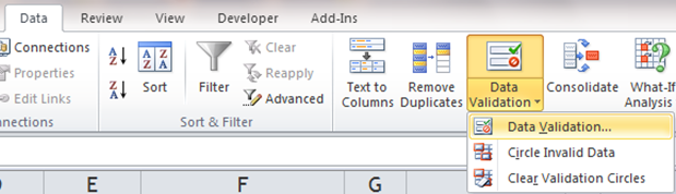 

5)    Under Settings, Allows: List, Source: =$K$3:$K$8 

OK. DONE!  You should be able to use the dynamic dropdown list you have just created.

One step further

Not all teachers are eligible to all classes.  e.g. only Iris and David are eligible to deliver Class F, would it be feasible to have only Iris and David on the dropdown list, in the ascending order of hours assigned?

Let’s talk about it in the next post.

Thanks to the many great articles on data validation by Debra Dalgleish who holds the excellent Contextures Blog.  This post is inspired by a recent post of Debra.

 

UPDATE: There will be a much simpler solution with Dynamic Array.  Check it out on my latest post – The power of Dynamic Arrays in #Excel 365