Usually we use vlookup for answering a particular question like “How many customers we had on January 1st 2014?” We expect an exact match and hence using FALSE as the last argument in the vlookup formula.
When do we use TRUE in vlookup then?
Assigning Grade according to scores is a typical example!

If we want to perform a vlookup using FALSE, we will need a table of at least 101 rows that lists the grade for each score from 0 to 100, like the one below:

wow… what a tedious work and a large table. Worse still, it cannot look up a score of e.g. 80.5 as this value is not in the table_array.
Here we go the TRUE vlookup with Approximate Match!
“If range_lookup is either TRUE or is omitted, an exact or approximate match is returned. If an exact match is not found, the next largest value that is less than lookup_value is returned.
Important If range_lookup is either TRUE or is omitted, the values in the first column of table_array must be placed in ascending sort order; otherwise, VLOOKUP might not return the correct value.” – From Excel Help
What this mean? Let’s take a look at the example below:
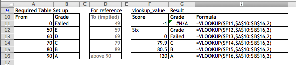
See how simple is the source data table.
Let’s look at cell F14 where the lookup_value is 79.9. As there is NO 79.9 in the 1st Column in the table_array, it returns the next largest value that is less than lookup_value, which is 70. And the corresponding result is “C”. Now it makes sense that the 1st column in the table_array has to be in ascending order, doesn’t it?
Remark:
- If the lookup_value is less than the smallest (1st) number in the 1st column of the table_array, it returns “#N/A”
- In cell F12 “Six” is input & the Header row in the tabel_array (A10:B16), the vlookup compares “Six” with “From”. As “Six” is larger than “From” but smaller than “0”, it returns “Grade”.
- Hint: AVOID include header row in assigning the table_array for TRUE vlookup, i.e. Use $A$11:$B$16 instead
Other examples for using TRUE vlookup:
Commission Table:

What is your case for using TRUE vlookup? Pls share with us by leaving a comment.


Hi All,
I’m looking for ab Excel formula solving the below:
I have list of account numbers in column A and in column B a list of charge methods associated to each account. One account can have a few charge methods associated – for example:
Account no Charge method A1 IC1 A1 IC2 A1 Exempt A2 IC1 A2 IC2 A3 IC1 A3 IC2 A3 IC3 A3 Exempt A4 IC1 A4 IC2 A4 Exampt
I would like to specify which account have at least one charge method “Exempt”. So for example: in column C value “Exempt” if if for A1 account “Exempt” is mentioned at least once in culumn B. I tried to use vlookup TRUE, but I’m not sure if it will be always accurate.
LikeLike
Hi Dorota,
Your question is not so clear to me…
Would you please further elaborate? or give some samples of your data; and stating what you intend to do.
Cheers,
LikeLike
Having a hard time with a lookup I am trying to set up. I have a column with 49,000 rows of phone numbers. I want to see if these phone numbers match another array of phone numbers I have. However my reference array of phone numbers only contains area-code and prefix, so only 6 digits. My lookup array contains full 9 digit numbers. So I want to see if the first 6 digits of those numbers match my reference array. So I’m looking for a partial match and having a hard time understanding where to put my wildcard characters to get the lookup to run properly. Any advice would be very appreciated.
LikeLike
Hi Ari,
To recap, do you mean:
1) Your lookup values contain 9 digits, but you need to lookup only the 1st 6 digits?
2) the values in the table array contains only 6 digits
If so, you may try sth like:
=COUNTIF(Ref_Range,LEFT(A1,6))
Hope it helps.
Cheers,
LikeLike
You may remove the area codes first using text to column before using vlook-up.. 🙂
LikeLike
Pingback: Nested IF to calculate credit rating
Pingback: Equation: equals number if another number is between a certain range
Pingback: Alternative to vlookup – Index and Match | wmfexcel
Pingback: vlookup – Text vs. Number | wmfexcel
Pingback: Tips in constructing vlookup | wmfexcel
Pingback: The basic of vlookup | wmfexcel
Pingback: vlookup with Match | wmfexcel